Black Marble HD: what a 30-meter output grid really adds

Work through the 500-to-30-meter grid ratio in a real Black Marble HD study, without confusing sharper output with independent night observations.

A coarse nighttime map becomes a much sharper-looking map in the four-panel figure below. Streets and coastal features are easier to distinguish in the final product. Has the satellite suddenly collected hundreds of times more independent nighttime observations?

The study’s method explains what changed. Its Black Marble HD workflow combined a 500-meter nighttime source-product grid with daytime and ancillary information to produce a 30-meter output grid. The sharper display is the result of that fusion. The grid spacing alone cannot tell us how many independent observations support it.

Using the real method figure from the 2019 Puerto Rico study by Román and colleagues, this article checks the inputs and works through the nominal grid arithmetic. The result is about 16.67 times as many grid intervals across a fixed distance, or a square-cell area ratio of about 277.78. Those are geometric ratios, not detector specifications or measured accuracy gains.

Read the four panels as a workflow

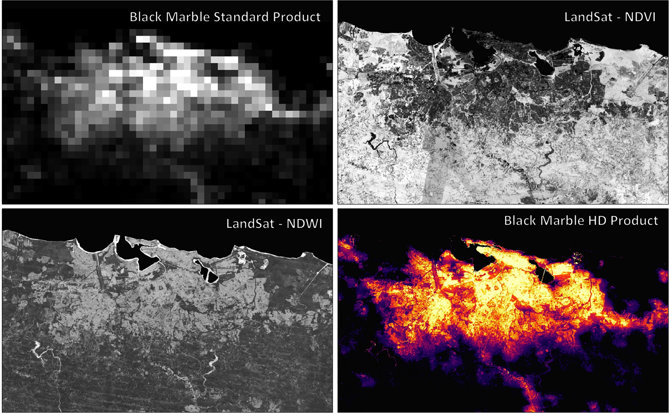
Full Figure 1 from the 2019 study. Upper left is a coarse Black Marble standard product, upper right Landsat NDVI, lower left Landsat NDWI, and lower right the more detailed fused Black Marble HD product. — The unchanged four-panel method figure. Panel locations here follow the embedded titles; the source caption reverses its upper-left and upper-right descriptions. Credit: Román et al. (2019), PLOS ONE 14(6): e0218883, Figure 1, CC0 source paper. Includes © OpenStreetMap contributors (ODbL). Open full-size figure

The upper-left panel shows the coarse Black Marble standard product. The upper-right and lower-left panels supply vegetation- and water-index views. The lower-right panel is the fused HD result, with much more visible spatial detail than the nighttime source panel alone.

This arrangement matters because the extra detail has a documented lineage. It did not all originate in a new set of fine-scale nighttime measurements. The figure is useful precisely because it lets a reader see the ingredients alongside the output.

Read the embedded panel labels in the published figure
Position	Embedded panel	What it contributes
Upper left	Black Marble Standard Product	Coarser nighttime-light source product
Upper right	Landsat NDVI	Daytime vegetation-index information
Lower left	Landsat NDWI	Daytime water-index information
Lower right	Black Marble HD Product	Fused output on a finer grid

The paper’s methods describe cubic-convolution resampling of the 500-meter nighttime product, combined with daytime surface-reflectance indices. OpenStreetMap roads also enter the visualization. In this historical workflow, the authors enhanced mapped roads to make them legible. A distinct line in the final display therefore needs to be read in the context of those inputs and transformations.

This account concerns the method in the 2019 paper. It does not assign the same workflow or characteristics to every present-day product carrying the Black Marble name.

Work through the 500-to-30 calculation

Nominal grid calculation using the study’s two product scales
Quantity	Calculation	Result	Interpretation
Source-product square cell	500 m × 500 m	250,000 m²	Nominal grid geometry
HD-output square cell	30 m × 30 m	900 m²	Nominal grid geometry
Across one dimension	500 ÷ 30	About 16.67	Ratio of grid spacings
By nominal square-cell area	250,000 ÷ 900	About 277.78	Area ratio; not independent observations

The nominal linear calculation is 500 divided by 30, giving approximately 16.67. Because a square has two dimensions, the corresponding area ratio is the square of that number: approximately 277.78. Equivalently, a nominal 500-meter square has an area of 250,000 square meters, while a nominal 30-meter square has an area of 900 square meters.

The non-integer ratio is worth keeping. A 500-meter width is not an exact multiple of 30 meters. Saying “278 cells inside each source cell” would suggest a precise nesting that this simple ratio does not establish. Grid origins, projections and resampling determine actual relationships between cells. Here, “about 278 times the nominal square-cell area” is the bounded geometric statement.

The 500-meter value is the source-product grid spacing used in this workflow. It is not being asserted as the native spatial resolution of the VIIRS Day/Night Band detector. Likewise, the 30-meter output spacing does not establish a new 30-meter nighttime sensor.

Why output cells are not independent evidence

Resampling makes values available on a different grid. Data fusion can add useful information about spatial structure from other inputs. Neither operation makes the number of output cells an automatic count of independently measured nighttime conditions.

That distinction affects how a map might be used downstream. If a reader treats every small output cell as a separate direct night observation, the map can appear to support a much more finely resolved conclusion than its observation lineage warrants. The area ratio is a helpful warning sign: it describes the expansion of the output grid, not a demonstrated multiplication of independent evidence.

For an analyst comparing products, two questions should therefore remain separate. How finely is the output represented? And what measurements and assumptions support a claim at that scale? The published figure answers part of the first and exposes important ingredients for the second.

Check the claim: “30-meter HD means 278 times more night measurements.”

The calculation compares nominal square-cell areas: 500² divided by 30² is about 277.78. The method resamples and combines information from several inputs. An area ratio does not count independent night measurements, and it does not quantify an accuracy improvement.

Why retain the coarser source panel when the HD map looks clearer?

Showing the source alongside the output helps the reader see which structure is present in the nighttime product and which detail is supported by daytime or ancillary inputs. It makes the visual improvement easier to interpret without confusing display detail with measurement independence.

The building-level boundary is explicit

The paper warns against using its HD retrievals to quantify outage conditions for individual buildings. That limit is consistent with the workflow distinction: a building-sized-looking feature in a rendered map does not by itself establish that building’s electricity status.

This article makes no new outage estimate, neighborhood comparison, household classification or recovery finding. It has not reconstructed the original raster processing. Its calculation uses only the two nominal product-grid scales, and its visual reading stays with the complete published method figure. It does not derive power use from the figure’s color palette.

The sharper result can still be valuable. Its value is clearer when the map’s legend and caption preserve the source-product grid, the fused output grid and the ancillary information. A good resolution claim should name all three before asking a reader to act on an individual pixel.

Sources and image use

Román et al. (2019), Satellite-based assessment of electricity restoration efforts in Puerto Rico after Hurricane Maria, PLOS ONE 14(6): e0218883. Methods section on Black Marble HD, Figure 1, and the authors’ individual-building limitation. The article is dedicated to the public domain under CC0.
OpenStreetMap copyright and ODbL attribution. The unchanged figure is reproduced with attribution to OpenStreetMap contributors because the described workflow uses mapped roads.