Launch Watch · Current evidence
Published
Smile’s 45-hour aurora watch: a test against its achieved orbit
A reproducible orbit model gives Smile 44.1 hours above its imaging gate. Compare that opportunity with the newly released aurora images.
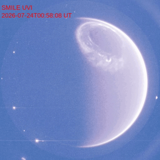
Smile’s newly released auroral images come with an unusually long observing claim: stretches of about 45 hours. ESA’s 30 September science announcement said readiness had been declared on 23 September; the accompanying ultraviolet sequence was recorded on 24 July. The release date and the observation date describe different events.
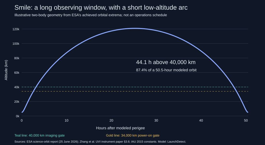
We tested the scale of that observing window against the mission’s reported achieved orbit. A simple two-body calculation gives about 44.1 hours above a 40,000-kilometre imaging gate in a 50.5-hour modeled revolution. That is a geometric opportunity. Actual usable observations also depend on instrument operation, pointing, calibration and data quality.
Start with the achieved orbit
ESA’s 25 June orbit report gives a high point 120,920 kilometres above the North Pole and a low point 5,027 kilometres over the South Pole. We treat those reported extrema as the apsides of an idealized ellipse. The spacecraft spends much longer near the high end, where its motion around Earth is slower, than near its close approach.
The inputs must be distances from Earth’s centre before applying the orbital equations. Adding the declared Earth radius to both altitudes gives radii of 127,298.1 and 11,405.1 kilometres. Their average is a semimajor axis of 69,351.6 kilometres. Using the altitudes alone would make a different, incorrect input to this model.
Two altitude gates make two different budgets
The UVI instrument paper, section 3.6, separates power-on and dark calibration at 34,000 kilometres from high-voltage auroral imaging at 40,000 kilometres. Applying both thresholds to the same idealized orbit keeps those activities from being counted as one continuous imaging period.
| Quantity | Calculated time | Meaning in this model |
|---|---|---|
| One revolution | 50.49 hours | Period calculated from reported extrema and stated constants |
| Above 34,000 km | 45.29 hours | Geometric interval above the paper’s power-on/calibration gate |
| Above 40,000 km | 44.12 hours | Geometric interval above the paper’s imaging gate |
| Between the two gates | 1.16 hours total | Difference between the two above-threshold intervals |
| Below 40,000 km | 6.37 hours total | Remainder of the modeled revolution |
The threshold crossings are also informative. In the model, altitude rises through 40,000 kilometres 3.18 hours after perigee and falls through it at 47.31 hours. The 44.12-hour interval between them occupies 87.4% of the modeled revolution. The two lower-altitude portions together account for the other 6.37 hours. This is a time budget for a stated geometric condition, not a log of when an instrument was commanded on.
By comparison, the prelaunch mission paper describes approximately 45 hours of ultraviolet observation in a 51-hour orbit. That rounded design ratio is 45 / 51 = 88.2%, leaving six hours. Keep it separate from our calculation. The roughly 0.9-hour difference between 45 and 44.12 is not an observed shortfall: one value is a rounded design description, the other follows from reported extrema and our simplified assumptions.
What the first images establish
The released ultraviolet sequence provides actual image evidence from a selected interval. It does not contain the complete 45-hour series needed to independently audit that duration. The geometric calculation cannot fill that gap: it predicts where the spacecraft could be, while the image documents a particular observation.
ESA’s September update also gives different instrument-specific states. UVI’s long auroral sessions are reported; SXI has taken calibration images, but Earth-pointed stray light remains excessive and adjustments are underway. An anticipated mid-October improvement is prospective. The update does not establish that the first good magnetopause X-ray image has already been obtained.
| Evidence | What it supports | What still needs another record |
|---|---|---|
| Reported achieved orbital extrema | Inputs for a simplified geometric model | The time-varying flight ephemeris and actual pointing |
| Released 24 July UVI scene | An actual selected ultraviolet image sequence | A complete calibrated 45-hour dataset with quality information |
| 30 September instrument update | The provider’s distinct UVI and SXI status reports | Independent validation of each instrument’s usable-data duty cycle |
For LaunchDetect readers, this distinction matters when comparing an observing mission’s first-light announcement with a coverage claim. A visually compelling image, an orbital opportunity and an accepted science product each answer a useful question. Substituting one for another can turn a credible first result into an unsupported availability promise.
Method: solve for the time at each threshold
We use an Earth radius of 6,378.1 kilometres and gravitational parameter of 398,600.4 cubic kilometres per second squared from IAU 2015 nominal terrestrial constants. Let ra and rp be the high and low centre distances. The semimajor axis is a = (ra + rp) / 2, and eccentricity is e = (ra − rp) / (ra + rp).
The period follows from T = 2π√(a3 / μ). At each threshold altitude, we add Earth’s radius and solve r = a(1 − e cos E). The elapsed fraction of the period is (E − e sin E) / 2π. Symmetry about apogee gives the interval above the threshold. The chart samples the resulting curve at 1,001 points; the threshold times use the analytic crossings rather than counting chart points.
Download both threshold crossings and durations, or download all 1,001 calculated altitude samples. Values with extra decimal places in the CSV support reproduction and are not statements of orbital measurement precision.
As a small sensitivity check, substituting the IAU nominal polar radius gives about 44.11 hours above 40,000 kilometres, roughly one minute less. The model omits a nonspherical Earth, perturbations, orbital evolution, pointing, radiation conditions and actual commanding. Those omissions matter more to a claim about realized science availability than this rounding-level radius choice. We also exclude a separate full-oval threshold whose distance convention is inconsistent between sections of the instrument paper.
The next useful evidence
The model makes the long northern observing arc plausible at the stated scale. To test a realized duty cycle, look for calibrated time sequences, quality flags and an explicit definition of usable observations. For SXI, the relevant next result is an Earth-pointed science image and the accompanying instrument assessment. Neither requirement can be replaced by counting the frames in the public auroral clip.
Sources and current-interest context
- ESA: Science begins for Smile, 30 September 2026.
- ESA: Smile reaches science orbit, 25 June 2026.
- Wang and colleagues: the Smile mission, 2025 prelaunch design.
- Zhang and colleagues: the Ultraviolet Imager, 2025, especially section 3.6. No paper figures are reproduced.
- ESA/CAS: first ultraviolet footage, scene from 24 July, released 30 September.
At the 4 October 2026, 20:04 UTC source check, ESA placed the science announcement in its Trending section and displayed 9,463 cumulative page views and 45 likes. These publisher-local counters explain the current-interest selection; they are not unique readers, recent growth, search volume or measured clicks.